# get required packages
import pandas as pdIn Financial Forecasting in Python, we will step into the role of CFO and learn how to advise a board of directors on key metrics while building a financial forecast, the basics of income statements and Balance Sheets, and cleaning messy financial data. During this blog we will examine real-life datasets from Netflix, Tesla, and Ford, using the pandas package. Following this blog we will be able to calculate financial metrics, work with assumptions and variances, and build our own forecast in Python.
1. Income statements
1.1 Tesla Motors Inc.
In this example we have chosen to download the latest Income Statemet from Tesla Motors Inc. as a csv file. Let’s have a look at our raw data:
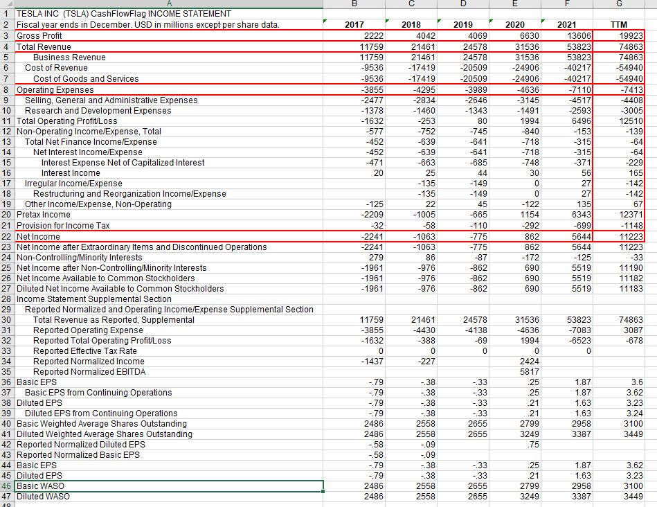
Tesla has a financial year end of 31 December and we have the results for the financial years 2017 to 2021, as well as an additional column headed TTM which stands for trailing twelve months which is the most recent 12 months of data available. We will be using this column together with the historical information to produce a forecast for the 2022 financial year. .
There are some problems with the data. We need to ensure the data is in the desire format and eliminate any headers we don’t want to use. This could be done manually of course but this would require editing the file every time we have new data. Much better to make use of Python, in particular the pandas library.
# load in our financials
income_statement = pd.read_csv('Data/Income Statement_Annual_As Originally Reported.csv')
Let’s focus our atttention on four key metrics - ‘Gross Profit’, ‘Total Revenue, ’Operating expenses’, and ‘Net Income’. To do this we’ll create a filtered income statement to only show these rows. The filtering code uses the following pattern.
dataframe[dataframe.columnname.isin(list_of_categories)]# Choose some interesting metrics
interesting_metrics = ['Total Revenue', 'Operating Expenses', 'Gross Profit', 'Net Income']
# Filter for rows containing these metrics
filtered_income_statement = income_statement[income_statement.metric.isin(interesting_metrics)]
# See the result
filtered_income_statement| metric | 2017 | 2018 | 2019 | 2020 | 2021 | TTM | |
|---|---|---|---|---|---|---|---|
| 0 | Gross Profit | 2222.0 | 4042.0 | 4069.0 | 6630.0 | 13606.0 | 19923.0 |
| 1 | Total Revenue | 11759.0 | 21461.0 | 24578.0 | 31536.0 | 53823.0 | 74863.0 |
| 5 | Operating Expenses | -3855.0 | -4295.0 | -3989.0 | -4636.0 | -7110.0 | -7413.0 |
| 19 | Net Income | -2241.0 | -1063.0 | -775.0 | 862.0 | 5644.0 | 11223.0 |
1.2 Forecasting revenue for Tesla
Let’s now append a new column with 2022 Forecast data, which we will assign the header “Forecast”. For this exercise, we would like to set the filtered_income_statement to only show the row ‘Revenue’.
Remember, the TTM column is the most recent 12-month value that we will use for the 2022 forecast. Thus far, we have the following information for 2022:
Total revenues for the 9 months to 30 September 2022 are 57,144 USD millions, up 58% on the 9 months to September 2021, so let’s ignore any seasonality and make a very crude estimate of revenue for 2022 for illustrative purposes of say 80,000 USD millions:
revenue_metric = ['Total Revenue']

# Filter for rows containing the revenue metric
filtered_income_statement = income_statement[income_statement.metric.isin(revenue_metric)]

# Get the number of columns in filtered_income_statement
n_cols = len(filtered_income_statement.columns)

# Insert a column in the correct position containing the column 'Forecast'
filtered_income_statement.insert(n_cols, 'Forecast', 80000)

filtered_income_statement| metric | 2017 | 2018 | 2019 | 2020 | 2021 | TTM | Forecast | |
|---|---|---|---|---|---|---|---|---|
| 1 | Total Revenue | 11759.0 | 21461.0 | 24578.0 | 31536.0 | 53823.0 | 74863.0 | 80000 |
Excellent, we successfully built a new table to include the 2022 forecast from a raw dataset.
2. Balance Sheet and forecast ratios
2.1 Calculating accounts receivable (debtors)
When we sell something on credit, the credit portion is in the balance sheet under ‘Accounts Receivable’ or ‘Debtors’. For example, if credit sales are made in January with a 60-day payback period, they would be recorded in our ‘Debtors’ account in January, but only be paid (released) in March, and so on.
In this exercise, we will create the following lists:
- The credit sales in the month
credits, which in this exercise is 60% of the sale value. - The total accounts receivable
debtors, to be calculated as the credits for the current month, plus the credits of the month before, minus the credits of two months before (as we assume the credits from 2 months ago or 60 days, will be repaid by then).
We have set an index for the variable month. The month value is set at 0.
# Create the list for sales, and empty lists for debtors and credits
month = 0
sales = [500, 350, 700]
debtors = []
credits = []

# Create the statement to append the calculated figures to the debtors and credits lists
for mvalue in sales:
    credits.append(mvalue * 0.6)
    if month > 0:
        debtors.append(credits[month] + credits[month-1])
    else:
        debtors.append(credits[month])
    month += 1
# Print the result
print("The ‘Debtors’ are {}.".format(debtors))
The ‘Debtors’ are [300.0, 510.0, 630.0].2.2 Bad debts
When offering credit terms to customers, there is always a risk that the customer does not pay their debt. In the finance world, this is known as “bad debts”.
As we have already recorded sales, we need to record the loss of sales now, as we never received the payment.
This affects both the income statement and the balance sheet. In the income statement, we record a negative value in the sales for the month we write off the debt. In the balance sheet, we need to reduce our debtor’s asset.
The following variables have been defined for January: debtors_jan = 1500
In February, we received news that a customer has gone into liquidation. This customer currently owes 500 USD.
We expect to recover 70% of this amount; the rest has to be written off as bad debts.
debtors_jan = 1500

# Calculate the bad debts for February
bad_debts_feb = 500 * 0.3

# Calculate the feb debtors amount
debtors_feb = (debtors_jan- bad_debts_feb)

# Print the debtors for January and the bad debts and the debtors for February
print("The debtors are {} in January, {} in February. February's bad debts are {} USD.".format(debtors_jan, debtors_feb, bad_debts_feb))
The debtors are 1500 in January, 1350.0 in February. February's bad debts are 150.0 USD.You can see that our debtors amount is reduced by the amount of bad debts.
2.3 Calculating accounts payable (creditors)
Now we will look at a scenario where we are the ones being granted credit. This means that we can buy something, but only have to pay for this amount later.
In this exercise, T-Z needs to buy nuts and bolts to produce 1000 units in January and 1200 units in February. The cost of nuts and bolts per unit is 0.25 USD. The credit terms are 50% cash upfront and 50% in 30 days.
Therefore, the creditors’ value, in this case, would be paid the month directly after. This means that the creditors’ value would only reflect the current month’s credit purchases.
# Set the cost per unit
unit_cost = 0.25

# Create the list for production units and empty list for creditors
production = [1000,1200]
creditors = []

# Calculate the accounts payable for January and February
for mvalue in production:
    creditors.append(mvalue * unit_cost * 0.5)

# Print the creditors balance for January and February
print("The creditors balance for January and February are {} and {} USD.".format(creditors[0], creditors[1]))
The creditors balance for January and February are 125.0 and 150.0 USD.As we can see, the Balance Sheet shows us what our real cash situation looks like, as just because we made a sale does not mean money in the bank, and incurring an expense also does not mean we have to pay it right away!
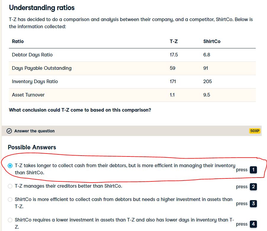
2.4 Debtor days ratio
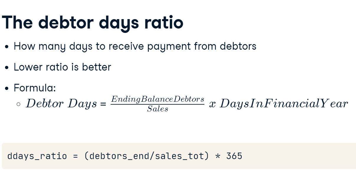
The first ratio we will look at is debtor days. This ratio looks at how many days it takes to receive our money from our debtors. It is usually calculated over a period of 1 financial year.
The following information is available to you:
- Sales for the year: 12,500 USD
- Ending Debtors balance: 650
# Create the variables
debtors_end = 650
sales_tot = 12500

# Calculate the debtor days variable
ddays_ratio = (debtors_end/sales_tot) * 365

# Print the result
print("The debtor days ratio is {}.".format(ddays_ratio))
The debtor days ratio is 18.98.2.5 Days payable outstanding
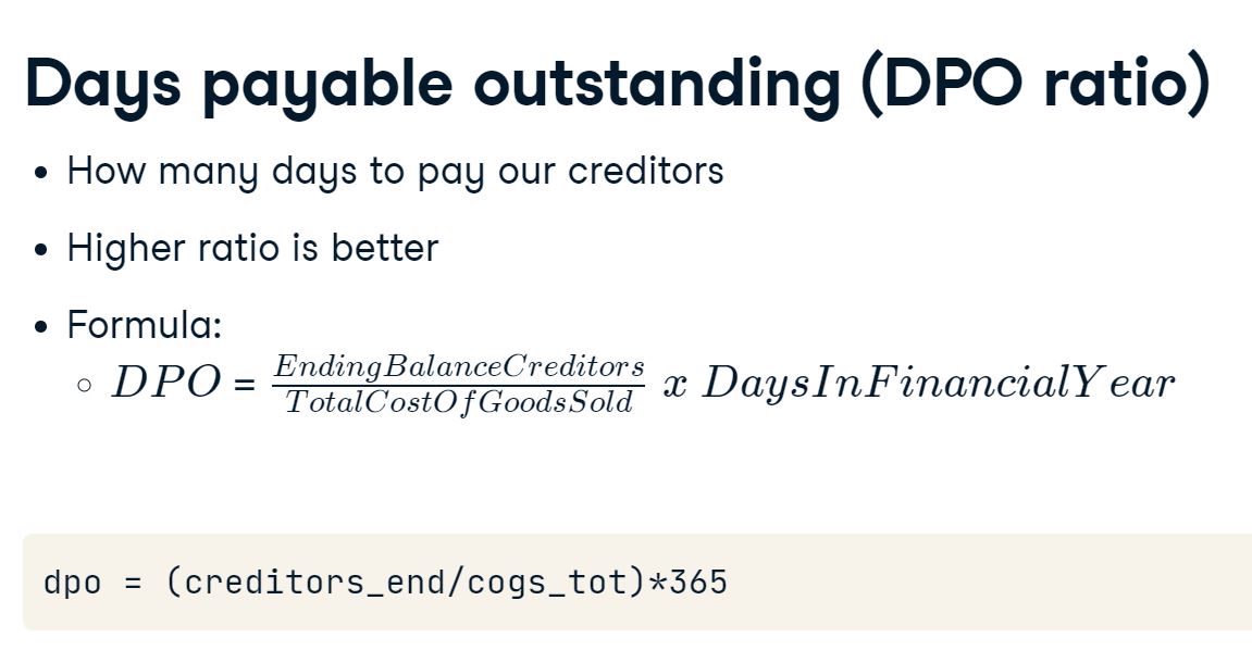
We will now have a look at our accounts payable, or creditors, and a ratio called the Days Payable Outstanding (DPO).
This ratio is an efficiency ratio that measures the average number of days a company takes to pay its suppliers.
T-Z wants to know its days payable outstanding and has asked you to calculate it.
# Get the variables
cogs_tot = 4000
creditors_end = 650

# Calculate the days payable outstanding
dpo = (creditors_end/cogs_tot)*365

# Print the days payable outstanding
print("The days payable outstanding is {}.".format(dpo))
The days payable outstanding is 59.3125.2.6 Days in inventory
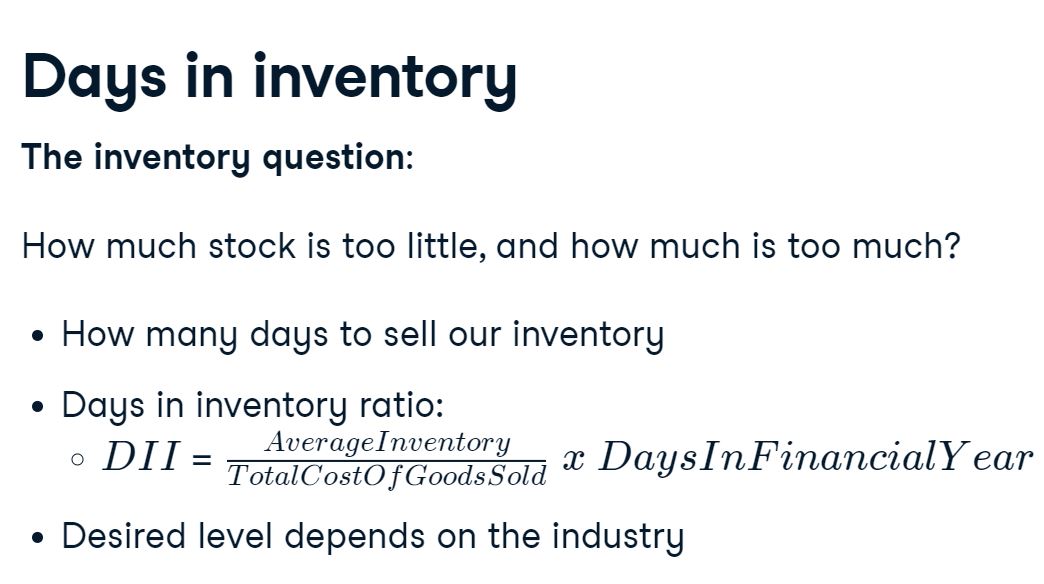
In this exercise, we will calculate the time it takes for a company to turn inventory into sales (days in inventory or DII ratio) based on the following information:
cogs_total = 4000
av_inv = 1900
sales_tot = 10000
ob_assets = 2000
cb_assets = 7000
# Calculate the dii ratio
dii_ratio = (av_inv/cogs_tot)*365
# Print the result
print("The DII ratio is {}.".format(dii_ratio))The DII ratio is 173.375.2.7 Asset Turnover
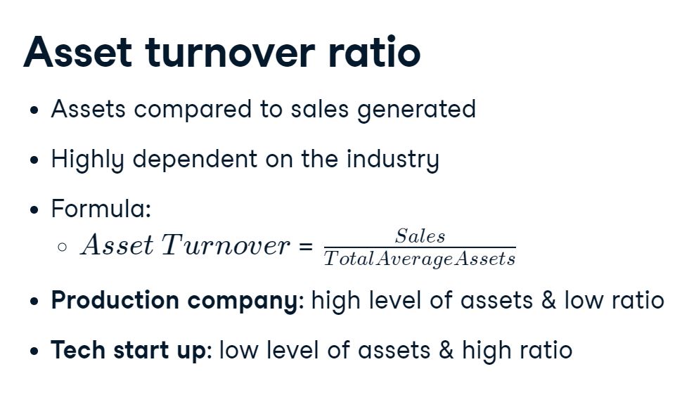
In this exercise, we will calculate the efficiency of a company’s assets by seeing how the company uses its assets to generate sales (asset turnover ratio):
# Calculate the Average Assets
av_assets = (ob_assets + cb_assets)/2

# Calculate the Asset Turnover Ratio
at_ratio = sales_tot/av_assets

# Print the Asset Turnover Ratio
print("The asset turnover ratio is {}.".format(at_ratio))
The asset turnover ratio is 2.2222222222222223.Let’s test our understanding of Balance Sheet ratios:
3. Balance Sheet
3.1 Calculating Balance Sheet ratios for Ford
Now we will look at a real life example, Ford Inc, a company producing motor vehicles. We will first upload a dataset: balance_sheet with the data for Ford Inc’s Balance Sheet as at 31 December 2017. The sales and cost of sales figures have been provided for 2017 within the Key_Figures_Memo dataset.
We are only interested in one line on the balance sheet, the Receivables (another name for Debtors), and therefore need to create a filter for this. In this exercise, we will use boolean indexing to filter our dataset for Receivables in the metric column. We will first specify our metric of interest ('Receivables'), and then check whether the column of interest has this value in each row. This will generate a boolean series of True and False values. With this series, we can then filter our existing dataset.
Once we have filtered our dataset, we can retrieve the receivables values from the most recent time period and calculate the debtor days ratio.
# read in the Ford Balance Sheet data
balance_sheet = pd.read_csv('Data/F-Balance-Sheet.csv')
# Create the filter metric for Receivables
receivables_metric = ['Receivables']
# Create a boolean series with your metric
receivables_filter = balance_sheet.metric.isin(receivables_metric)
# Use the series to filter the dataset
filtered_balance_sheet = balance_sheet[receivables_filter]
filtered_balance_sheet | metric | 2013-12 | 2014-12 | 2015-12 | 2016-12 | 2017-12 | |
|---|---|---|---|---|---|---|
| 6 | Receivables | 87309.0 | 92819.0 | 101975.0 | 57368.0 | 62809.0 |
# bring in values for Sales and Cost of Sales
sales=156776
cogs=131332
# From previous step
receivables_metric = ['Receivables']
receivables_filter = balance_sheet.metric.isin(receivables_metric)
filtered_balance_sheet = balance_sheet[receivables_filter]
# Extract the zeroth value from the last time period (2017-12)
debtors_end = filtered_balance_sheet['2017-12'].iloc[0]
# Calculate the debtor days ratio
ddays = (debtors_end/sales) * 365
# Print the debtor days ratio
print("The debtor day ratio is {:.0f}. A higher debtors days ratio means it takes longer to collect cash from debtors.".format(ddays))The debtor day ratio is 146. A higher debtors days ratio means it takes longer to collect cash from debtors.Next, we will learn how to append this information into our forecast.
3.2 Forecasting the Balance Sheet for Ford
Now that we have the ratios for Ford, the management wishes to improve them for the 2018 financial year.
There is one ratio in particular that management would like to be improved – the debtor days ratio, which is currently sitting at 146 days, while better than Nissan (244 days), is still much higher than Toyota, the industry leader (31 days).
Management would like to bring the debtor days down to below 100 days.
# set target debtor days
ddays = 99
Sales are expected to increase by 10%. Calculate these forecasted sales, f_sales from the existing sales :
# Calculate the forecasted sales
f_sales = sales * 1.10
f_sales172453.6We can rearrange the debtor days formula to calculate the closing balance of debtors needed to achieve 99 debtor days :
# Solve for the forecasted debtors' ending balance
f_debtors_end = f_sales * ddays/ 365

print("If sales rise by 10% and the debtor days decrease to {:.0f} then the forecasted closing balance for debtors will be {:.0f}.".format(ddays, f_debtors_end))
If sales rise by 10% and the debtor days decrease to 99 then the forecasted closing balance for debtors will be 46775.Let’s now append a column to include the forecasted debtors:
# Get the number of columns in the filtered balance sheet
n_cols = len(filtered_balance_sheet.columns)

# Append a Forecast column of the forecasted debtors' end balance
filtered_balance_sheet.insert(n_cols, 'Forecast', f_debtors_end)

# See the result
filtered_balance_sheet| metric | 2013-12 | 2014-12 | 2015-12 | 2016-12 | 2017-12 | Forecast | |
|---|---|---|---|---|---|---|---|
| 6 | Receivables | 87309.0 | 92819.0 | 101975.0 | 57368.0 | 62809.0 | 46775.086027 |
4. Financial periods and how to work with them
4.1 Converting quarters into months
A company has a challenge in separating data into months. It has received the following data:
- Quarter 1 = 700
- Quarter 2 = 650
The split across the months within each quarter is equal. Our goal is to separate this data into a list format containing the amounts per month for the first two quarters.
# Create a list for quarters and initialize an empty list qrtlist
quarters = [700, 650]
qrtlist = []

# Create a for loop to split the quarters into months and add to qrtlist
for qrt in quarters:
 month = round(qrt / 3, 2)
 qrtlist = qrtlist + [month, month, month]

# Print the result
print("The values per month for the first two quarters are {}.".format(qrtlist))
The values per month for the first two quarters are [233.33, 233.33, 233.33, 216.67, 216.67, 216.67].4.2 Merging months into quarters
Now we saw what to do when we wanted to split quarters into months for more detailed monthly information. But what happens when the opposite is true and we wish to combine data into fewer columns? This is typical when dealing with historical data, when monthly details may not be necessary, or when we need a highly consolidated version of the data for a report.
The key here is to create an index, and then only add to the quarter total quarter in cycles of 3, or until the length of the list. We can do this with the following code:
if index % 3 == 0 or index == len(months):This code checks whether the index divided by three yields a remainder of 0, or if the index is at the end of the list months. Thus, in a loop it will execute the specified code every three months or when it reaches the end of the list.
The monthly sales are already provided in the code as months, containing the sales from the first two quarters, as well as the first month of Q3. Our task is to generate a new list called quarters that contains the quarterly totals from the first three months (which includes the partial total of Q3).
# Create a months list, as well as an index, and set the quarter to 0
months = [100, 100, 150, 250, 300, 10, 20]
quarter = 0
quarters = []
index = 1

# Create for loop for quarter, print result, and increment the index
for sales in months:
    quarter += sales
    if index % 3 == 0 or index == len(months):
        quarters.append(quarter)
        quarter = 0
    index = index + 1

print("The quarter totals are Q1: {}, Q2: {}, Q3: {}".format(quarters[0], quarters[1], quarters[2]))
The quarter totals are Q1: 350, Q2: 560, Q3: 20Let’s have a look at a library that can help us more when working with dates.
4.3 The datetime library
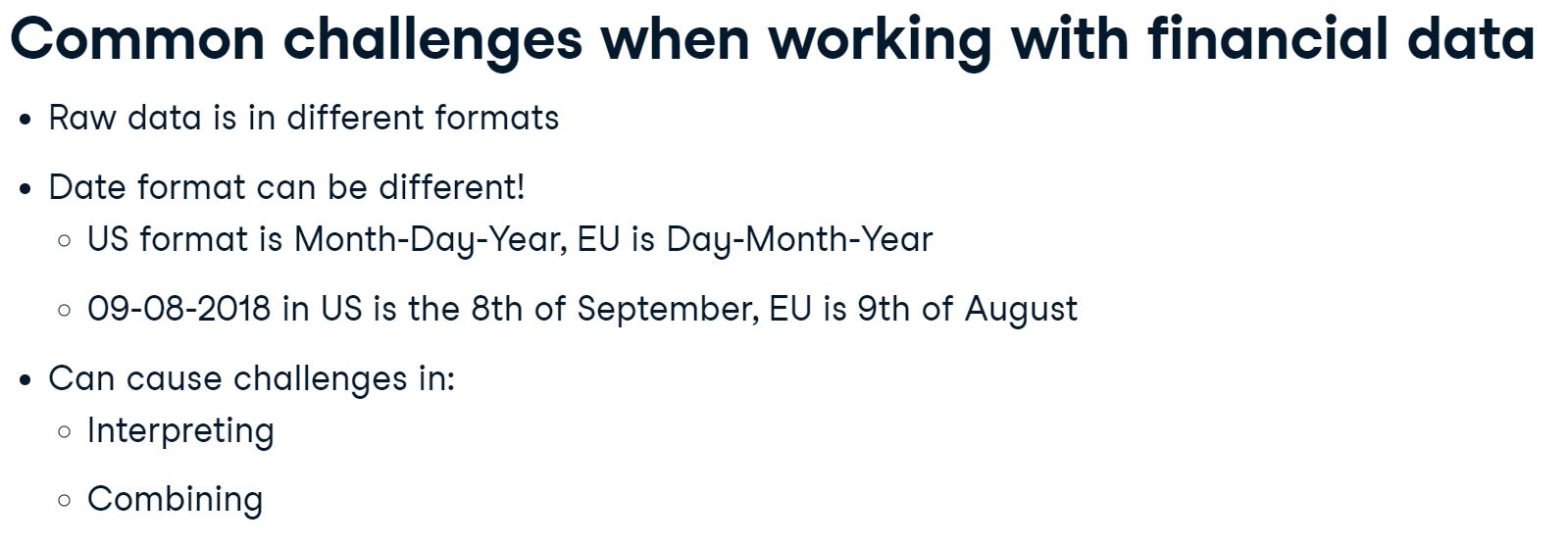
Sales area A in Europe and Sales area B in Australia have different date formats.
- Sale A: 4000 on 14/02/2018
- Sale B: 3000 on 2 March 2018
If we want to consolidate or compare sales periods, we need to convert to the same date format. We can easily do this by using the datetime library and the datetime.strptime(date_string, format) method, using the following directives:
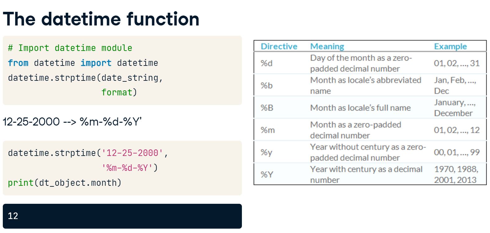
# Import the datetime python library
from datetime import datetime

# Create a dt_object to convert the first date and print the month result
dt_object1 = datetime.strptime('14/02/2018', '%d/%m/%Y')
print(dt_object1)

# Create a dt_object to convert the second date and print the month result
dt_object2 = datetime.strptime('2 March 2018', '%d %B %Y')
print(dt_object2)
2018-02-14 00:00:00
2018-03-02 00:00:004.4 Converting date formats - explicit
Let’s revisut one of the dates from the previous exercise.
- Sale A: 4000 on 14/02/2018
We used the datetime library to identify the day d, month m, and year y which could help us to identify data from datasets with different date formats. However, what about a scenario where we want to convert date formats into a specific format?
In this exercise we will convert Sale A from the format 14/02/2018 to the same date format as Sale B (i.e. 14 February 2018).
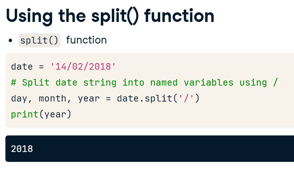
We can do this easily with built-in Python functions. To split a string we can use the .split()method:

# Set the variable for the datetime to convert
dt = '14/02/2018'

# Create the dictionary for the month values
mm = {'01': 'January', '02': 'February', '03': 'March'}

# Split the dt string into the different parts
day, month, year = dt.split('/')

# Print the concatenated date string
print(day + ' ' + mm['02'] + ' ' + year)
14 February 20185. Tips and tricks when working with datasets
5.1 Working with datasets - month totals
In this exercise, we will be exploring a dataset that has multiple sales in one month. We will create a script that will enable us to identify dates within the same month, and combine them into a new month total, and append this to the table.
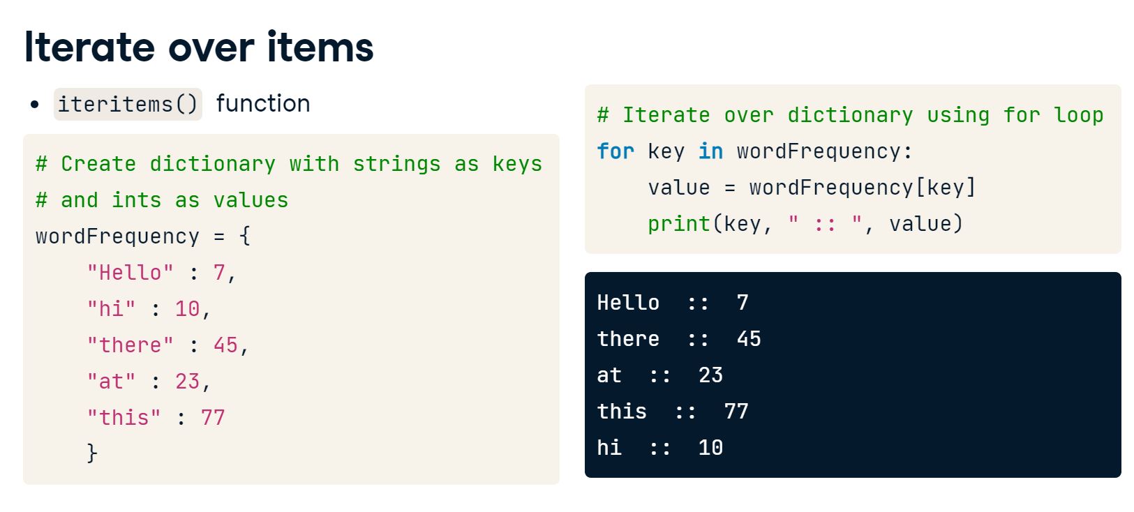
We will be using the dataset df, which represents data from one of our sales areas. Print it out in the console to have a look at the data. As you can see, there were two sales in March. We will combine these sales into a single month total. We can iterate over the dataset using the .iteritems() method.
We will also be using the .split() method.
# create a DataFrame to include our sales data
df = pd.DataFrame(columns=['Description','14-Feb', '19-Mar', '22-Mar'])

df.loc[0] = ['Sales', 3000, 1200, 1500]
df| Description | 14-Feb | 19-Mar | 22-Mar | |
|---|---|---|---|---|
| 0 | Sales | 3000 | 1200 | 1500 |
# Set the index to start at 0
index = 0

# Create the dictionary for the months
tt = {'Jan': 0, 'Feb': 0, 'Mar': 0}
# Create a for loop that will iterate the date and amount values in the dataset
for date, amount in df.iteritems():
# Create the if statement to split the day and month, then add it to the new tt variable
if index > 0:
day, month = date.split('-')
tt[month] +=float(amount[0])
index += 1
print(tt){'Jan': 0, 'Feb': 3000.0, 'Mar': 2700.0}/tmp/ipykernel_127/3317898835.py:2: FutureWarning: iteritems is deprecated and will be removed in a future version. Use .items instead.
for date, amount in df.iteritems():5.2 Working with datasets - combining datasets
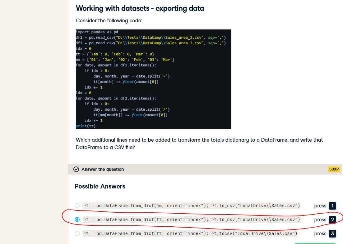
In this example, we will be working with two datasets, df1 and df2. You will notice that they contain different date formatting.
More specifically, df1 specifies the month by the name (e.g. 02-Feb-18), whereas df2 specifies the month numerically (e.g. 06/01/2018). Additionally, df1 uses a hyphen (-) as a separator, whereas df2 uses a forward slash (/) as a separator.
We will be combining these two datasets to form a consolidated forecast for the quarter. To do this, we will need to parse the different date formats of df1 and df2.
# create a DataFrame to include our sales data
df1 = pd.DataFrame(columns=['02-Feb-18', '15-Mar-18'])

df1.loc[0] = [3000, 1200]
df1| 02-Feb-18 | 15-Mar-18 | |
|---|---|---|
| 0 | 3000 | 1200 |
# create an empty dictionary containing total sales for each month initialized to 0
totals = {'Jan': 0, 'Feb': 0, 'Mar': 0}

# create a dictionary containing the months (Jan, Feb, Mar) and corresponding numbers
calendar = {'01': 'Jan', '02': 'Feb', '03': 'Mar'}
# Create a for loop to iterate over the items in the first dataset df1
for date, amount in df1.iteritems():
day, month, year = date.split('-')
totals[month] +=float(amount[0]) /tmp/ipykernel_127/1296325721.py:2: FutureWarning: iteritems is deprecated and will be removed in a future version. Use .items instead.
for date, amount in df1.iteritems():# create a DataFrame to include our sales data
df2 = pd.DataFrame(columns=['06/01/2018', '14/02/2018'])
df2.loc[0] = [1000, 1200]
df2| 06/01/2018 | 14/02/2018 | |
|---|---|---|
| 0 | 1000 | 1200 |
# Create a for loop to iterate over the items in the second dataset df2
# This time month will yield a a numerical reference, so we will need to use our calendar dictionary to add the amount to our totals dictionary.
for date, amount in df2.iteritems():
        day, month, year = date.split('/')
        totals[calendar[month]] += float(amount[0])

print(totals)
{'Jan': 1000.0, 'Feb': 4200.0, 'Mar': 1200.0}/tmp/ipykernel_127/4206160929.py:3: FutureWarning: iteritems is deprecated and will be removed in a future version. Use .items instead.
for date, amount in df2.iteritems():5.3 Exporting data
6. Assumptions and variances in forecasts
6.1 Building sensitive forecast models
6.2 Weighted probability
Txs Tools, a company selling hardware tools, is looking to expand out of their home market A into Market B. They have done some market research, and have received the following numeric probabilities:
Txs Tools will only be motivated to expand if they can have reasonable assurance that they will achieve sales of 400 or more. To manage the different forecast sales probabilities, Txs Tools have asked us to calculate the weighted probability.
# Create the combined list for sales and probability
sales_probability = ['0|0.05', '200|0.10', '300|0.40', '500|0.2', '800|0.25']
weighted_probability = 0

# Create a for loop to calculate the weighted probability
for pair in sales_probability:
    parts = pair.split('|')
    weighted_probability += float(parts[0]) * float(parts[1]) # float converts to a floating point

# Print the weighted probability result
print("The weighted probability is {}.".format(weighted_probability))
The weighted probability is 440.0.Have a look at the calculated weighted probability. We can see it reflects a weighted value between the highest and lowest sales figures. The weighted probability is a technique to manage the uncertainty in Txs Tools sales forecasting, and can give a more balanced view on expected sales numbers as opposed to just going for the lowest or highest number.
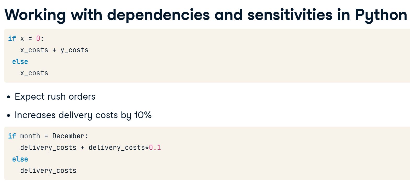
6.3 Market sentiment
Txs Tools has forecast sales of 500 in January, with an expected increase of 5% per month for the rest of the quarter.
However, this is dependent on the market sentiment. Based on historical trends, the following information has been provided:
- If the market sentiment drops below 0.6 then the sales will only be realized at an increase of 2% per month.
- If market sentiment increases above 0.8. then sales are expected to increase by 7%.
# Create the computevariance function
def computevariance(amount, sentiment):
 if (sentiment < 0.6):
  res = amount + (amount * 0.02)
 elif (sentiment > 0.8):
  res = amount + (amount * 0.07)
 else:
  res = amount + (amount * 0.05)
 return res
# Compute the variance for jan, feb and mar
jan = computevariance(500, 0.5)
feb = computevariance(500, 0.65)
mar = computevariance(500, 0.85)
print("The forecast sales considering variance due to market sentiment is {} for Jan, {} for Feb, and {} for Mar.".format(jan, feb, mar))The forecast sales considering variance due to market sentiment is 510.0 for Jan, 525.0 for Feb, and 535.0 for Mar.6.4 Dependencies and sensitivity
6.5 Assigning dependencies for sales and COGS
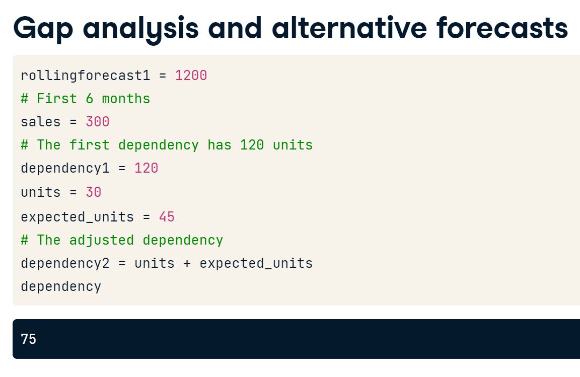
Txs Tools have built a monthly forecast for their gross profit. This will rely on dependencies for Sales and COGS.
Set the dependencies for sales and cogs based on the information below:
Sales dependency
sales_dep: The sale price is the net price after 1 USD commission. Commissions paid increase from 1 USD per unit to 2 USD per unit for every unit above 350 units sold.Cost dependency
cost_dep: When sales per unit increase above 500 units, an additional production line needs to be used, causing an increase in the cost per unit above 500 of 2 USD per unit.
The baseline sale price per unit (base_sales_price) is 15 USD and the baseline cost per unit (base_cost_price) is 7 USD.
# instantiate the base sales price
base_sales_price = 15

# instantiate the sales
sales = 750
# Set the Sales Dependency
if sales >= 350:
sales_dep = (350 * base_sales_price) + ((sales - 350) * (base_sales_price - 1))
else:
sales_dep = sales * base_sales_price
# Print the results
print("The sales dependency is {} USD.".format(sales_dep))The sales dependency is 10850 USD.# instantiate the bases cost price
base_cost_price = 7# Set the Cost Dependency
if sales >= 500:
cost_dep = (500 * base_cost_price) + ((sales - 500) * (base_cost_price + 2))
else:
cost_dep = sales * base_cost_price
# Print the results
print("The cost dependency is {} USD.".format(cost_dep))The cost dependency is 5750 USD.6.6 Building a sensitivity analysis for gross profit
xs Tools is now ready to use these dependencies in the gross profit forecast.
The following forecast unit sales have been provided:
Jul = 700 Aug = 350 Sep = 650The dependencies for sales and cogs are based on the following:
Sales dependency
sales_dep: The sale price is the net price after 1 USD commission. Commissions paid increase from 1 USD per unit to 2 USD per unit for every unit above 350 units sold.Cost dependency
cost_dep: When sales per unit increase above 500 units, an additional production line needs to be used, causing an increase in the cost per unit above 500 of 2 USD per unit.
The basic cost price base_cost_price = 7 and basic sales price base_sales_price = 15
# Create the sales_usd list
sales_usd = [700, 350, 650]
# Create the if statement to calculate the forecast_gross_profit
for sales in sales_usd:
if sales > 350:
sales_dep = (350 * base_sales_price) + ((sales - 350) * (base_sales_price - 1))
else:
sales_dep = sales * base_sales_price
if sales > 500:
cost_dep = (500 * base_cost_price) + ((sales - 500) * (base_cost_price + 2))
else:
cost_dep = sales * base_cost_price
forecast_gross_profit = sales_dep - cost_dep
# Print the result
print("The gross profit forecast for a sale unit value of {} is {} USD.".format(sales, forecast_gross_profit))The gross profit forecast for a sale unit value of 700 is 4850 USD.
The gross profit forecast for a sale unit value of 350 is 2800 USD.
The gross profit forecast for a sale unit value of 650 is 4600 USD.6.7 Assigning dependencies for expenses
Txs Tools wants to assign a dependency for its operating expenses, particularly admin salaries.
The conditions are as follows:
Admin expenses increase in July and August (
JulandAug) as temporary workers need to be hired to cover the summer holiday.The increase is based on the number of employees taking holidays during that time. For the current year, the value for August is
emp_leave= 6 (6 employees expected to take leave).The cost is 80 USD per temp employee hired.
# instantiate the emp leave value for August
emp_leave = 6
# Set the admin dependency
if emp_leave > 0:
admin_dep = emp_leave * 80
# Print the results
print("The admin dependency for August is {} USD.".format(admin_dep))The admin dependency for August is 480 USD.6.8 Build a sensitivity analysis for the net profit
Txs Tools has provided the following forecast admin cost in USD based on full-time employees:
Jul = 1500 Aug = 1500 Sep = 1500Build the forecast net profit forecast_net_profit when emp_leave = [6, 6, 0] and the cost per temp employee is 80 USD.
# instantiate our standing data
admin_usd = [1500, 1500, 1500]
emp_leave = [6, 6, 0]
forecast_gross_profit = [4850, 2800, 4600]
# Create an index variable and initialize this index to 0
index = 0
# Create the dependency by looping through the admin_usd list, using our index to access the correct month in our lists.
for admin in admin_usd:
temp = emp_leave[index]
if temp > 0:
admin_dep = temp * 80 + admin
else:
admin_dep = admin
forecast_net_profit = forecast_gross_profit[index] - admin_dep
print(forecast_net_profit)
index += 1
print("The forecast net profit is: {} USD.".format(forecast_net_profit))2870
820
3100
The forecast net profit is: 3100 USD.6.9 Working with variances in the forecast
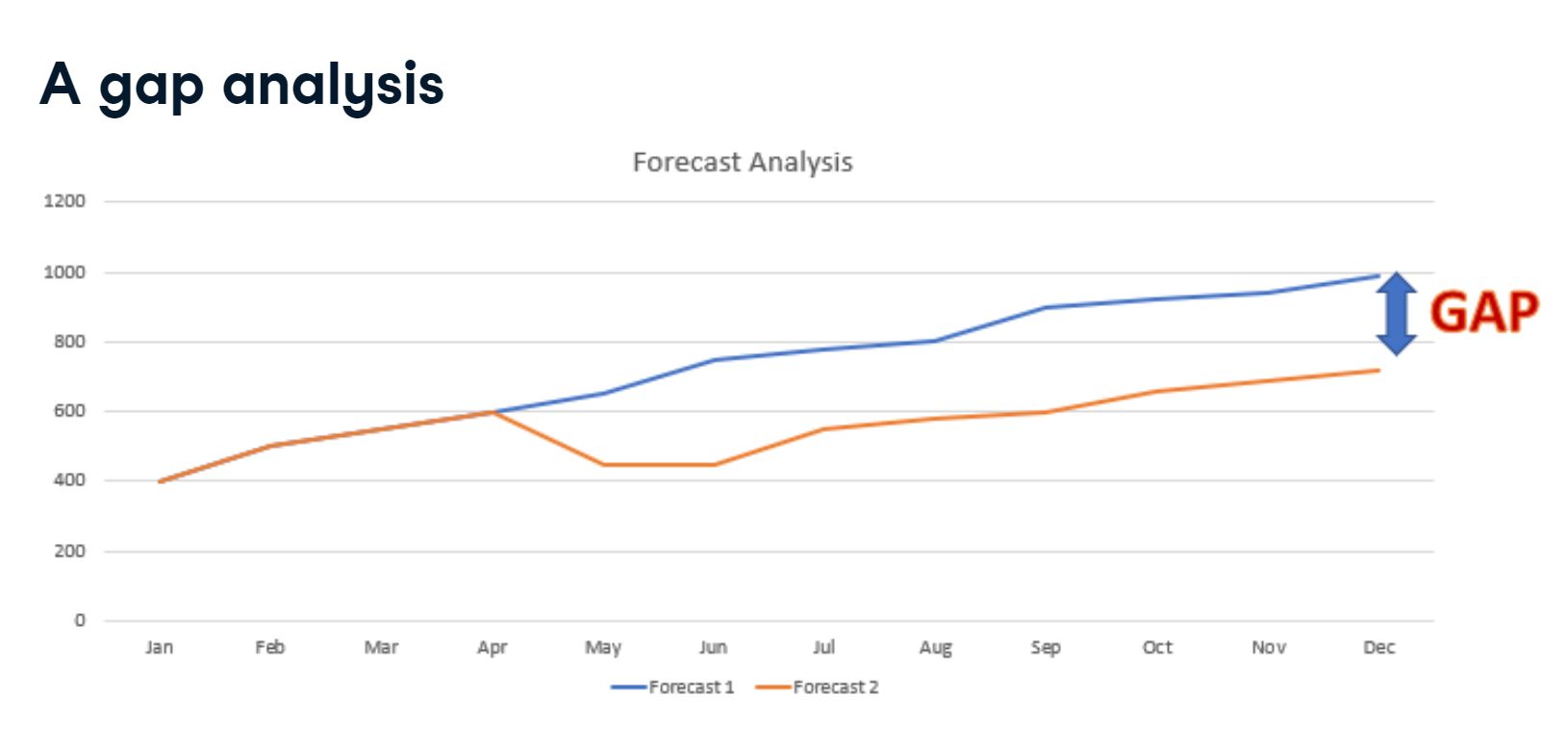
Identifying, quantifying, and investigating the difference between an old forecast and the new forecast is often referred to as Gap Analysis.
Building an alternate forecast
We will now build an alternative forecast for Txs Tools. The new quarter forecast is based off actual data for Jul - Aug as well as adjusted forecast data for September. The data (units sold) is as follows:
- Jul = 700
- Aug = 220
- Sep = 520
The dependencies calculations have already been completed from the previous exercise. The following information applies:
- base_cost_price = 7
- base_sales_price = 15
# create a dependencies() function for sales and costs with the arguments base_cost_price,base_sales_price, and sales_usd
# Pass the arguments into the function in this order.

def dependencies(base_cost_price, base_sales_price, sales_usd):
    res = []
    for sales in sales_usd:
        if sales >= 350:
            sales_dep = (350 * base_sales_price) + ((sales - 350) * (base_sales_price - 1))
        else:
            sales_dep = sales * base_sales_price
        if sales >= 500:
            cost_dep = (500 * base_cost_price) + ((sales - 500) * (base_cost_price + 2))
        else:
            cost_dep = sales * base_cost_price
        res.append(sales_dep - cost_dep)
    return res
# Create scenario forecast1 for the original forecast
forecast1 = dependencies(7, 15, [700, 350, 650])
# Create scenario forecast2 for the alternative forecast.
# Use the data provided above to calculate the alternative forecast
forecast2 = dependencies(7, 15, [700, 220, 520])print("The original forecast scenario is {}:".format(forecast1))
print("The alternative forecast scenario is {}:".format(forecast2))The original forecast scenario is [4850, 2800, 4600]:
The alternative forecast scenario is [4850, 1760, 3950]:6.10 Building a gap analysis between forecasts
Txs Tools now has two forecasts, the original forecast forecast1 and the adjusted forecast forecast2.
The dependencies have already been defined as def dependencies(base_cost_price, base_sales_price, sales_usd), where base_cost_price = 7 and base_sales_price = 15, with forecast2 based off the following adjusted sales unit values:
- Jul = 700
- Aug = 220
- Sep = 520
In this exercise, we will look at how to use a for loop to cycle between two different lists, forecast1 and forecast2 and calculate the difference (“gap”) using an incremented index. It is possible to do this simultaneously as both lists have the same length.
# Set the two results
forecast1 = dependencies(7, 15, [700, 350, 650])
forecast2 = dependencies(7, 15, [700, 220, 520])

# Create an index and the gap analysis for the forecast
index = 0
for value in forecast2:
    print("The gap between forecasts is {}".format(value - forecast1[index]))
    index += 1
The gap between forecasts is 0
The gap between forecasts is -1040
The gap between forecasts is -650You can see how easy it is to use a for loop to compare results across different lists.
Note that the gap between forecasts is driven purely by the difference in sales volume - base sales and cost prices are unchanged.
In July forecast2 sales are as per forecast 1 - so no gap.
In August forecast2 sales are 220 units against 350 - resulting in a gap of 130 units x profit per unit of 8 (15 - 7) which is 1040
In September forecast2 sales are 520 units against 650 - resulting in a gap of 130 units x profit per unit of 8 (15 - 7) which is 1040, but we also have a saving of 3 per unit (sales commission 1 and additional production line cost 2) which reduces the gap by 130 x 3 = 390 to 650.
6.11 Setting dependencies for Netflix
Netflix compiled a forecast up to the 2019 financial year netflix_f_is, and has based the sales figures in 2019 on the following dependency:
- Number of active subscriptions, which are based on the success of Netflix original shows.
For 2019, the success of original shows (critical and commercial acclaim) are estimated at 78%. The total amount of subscribers per percentage point is 500, and set to the variable n_subscribers_per_pp (i.e there is a calculated correlation between show success and number of subscribers).
In this exercise, we will calculate how dependent sales are on the number of subscribers in the forecast, which we will use in the next exercise.
# instantiate subscribers per % point
n_subscribers_per_pp = 500

# load in Netflix financials
netflix_f_is = pd.read_csv('Data/Netflix.csv')
netflix_f_is| metric | 2014_act | 2015_act | 2016_act | 2017_fc | 2018_fc | 2019_fc | |
|---|---|---|---|---|---|---|---|
| 0 | Sales | 5505 | 6780 | 8831 | 11688 | 14979 | 17994 |
| 1 | EBITDA | 528 | 493 | 611 | 1088 | 1899 | 2943 |
| 2 | Operating profit (EBIT) | 403 | 306 | 380 | 837 | 1660 | 2702 |
| 3 | Net income | 267 | 123 | 187 | 559 | 1024 | 1721 |
# Create a filter to select the sales row from the netflix_f_is dataset
sales_metric = ['Sales']

# Filter for rows containing the Sales metric
filtered_netflix_f_is = netflix_f_is[netflix_f_is.metric.isin(sales_metric)]

# Extract the 2019 Sales forecast value
forecast1 = netflix_f_is['2019_fc'].iloc[0]

# Print the resulting forecast
print("The sales forecast is {}.".format(forecast1))
The sales forecast is 17994.# Set the success percentage to 78%
pct_success = 0.78
# Calculate the dependency for the subscriber base
n_subscribers = n_subscribers_per_pp * pct_success
# See the result
print("The dependency for the subscriber base is {}.".format(n_subscribers))The dependency for the subscriber base is 390.0.# Calculate the ratio between forecast sales and subscribers
sales_subs_ratio = forecast1 / n_subscribers
# See the result
print("The ratio between subscribers and sales is 1 subscriber equals ${:.2f}.".format(sales_subs_ratio))The ratio between subscribers and sales is 1 subscriber equals $46.14.6.12 Calculating an alternative forecast for Netflix
The original assumptions are as follows: the total amount of subscribers at a 78% success rate results in 39,000 subscribers. We used this to build the forecast numbers.
However, the success rate for 2019 has been recalculated to have a probability of 65%, and the management has asked us to make an adjusted forecast based on this value.
The ratio between the subscribers and sales is 1 subscriber to 0.46 USD sales, set to variable sales_subs_ratio.
# instantiate sales subs ratio
sales_subs_ratio = 0.46
# Set the proportion of successes to 65%
pct_success2 = 65
# Calculate the number of subscribers
n_subscribers2 = n_subscribers_per_pp * pct_success2
# Calculate the new forecast
forecast2 = n_subscribers2 * sales_subs_ratio
forecast214950.0# Insert a column named AltForecast, containing forecast2
filtered_netflix_f_is.insert(len(filtered_netflix_f_is.columns), 'AltForecast', forecast2)
# Insert a column named Gap, containing the difference
filtered_netflix_f_is.insert(len(filtered_netflix_f_is.columns), 'Gap', forecast1 - forecast2)
# See the result
filtered_netflix_f_is| metric | 2014_act | 2015_act | 2016_act | 2017_fc | 2018_fc | 2019_fc | AltForecast | Gap | |
|---|---|---|---|---|---|---|---|---|---|
| 0 | Sales | 5505 | 6780 | 8831 | 11688 | 14979 | 17994 | 14950.0 | 3044.0 |
Key takeaways
We learned how to harnass Python, and in particular the pandas library to wrangle raw financial data, and extract relevant information to calculate key metrics.
We also learned how to handle date inconsistencies using the datetime library, parse dates using the split() method, and how to automate our work by writing functions and using for loops and .iteritems.
Automating the financial forecasting process allows fast iterations over different scenarios, saving time and reducing the scope of manual error.